Introduction
The final projects explored some interest methods of manipulation, including the image quilting algorithm for texture synthesis and transfer, and the gradient domain processing technique widely used in blending, tone-mapping, and non-photorealistic rendering.
Image Quilting
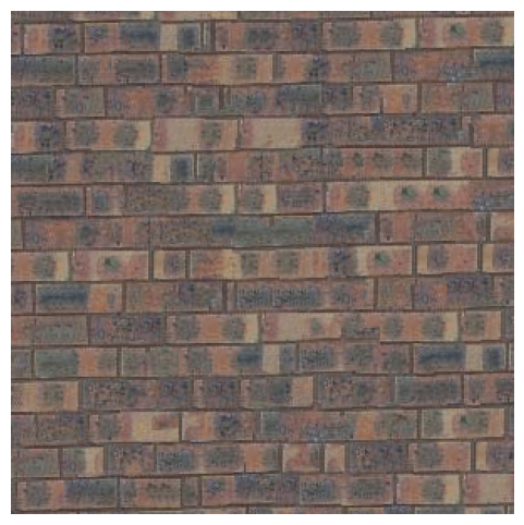
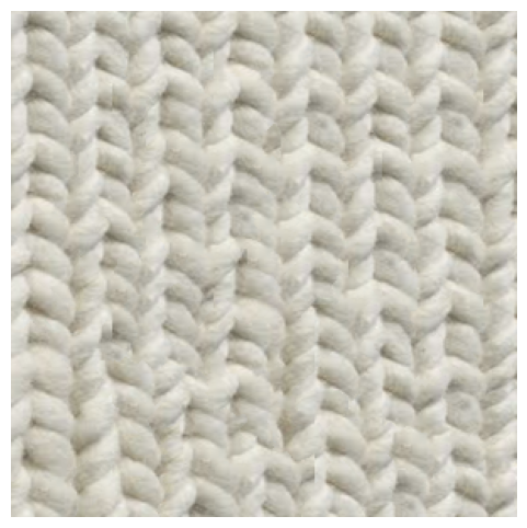
A texture is an image's structure of colors and intensities. The image quilting algorithm aims to achieve both texture synthesis, creating texture images larger than the original small samples, and texture transfer, preserving the shape of the image while changing the overall texture.
Randomly Sampled Textures
To start synthesize target texture images from a single source sample, I implemented a naive function quilt_random(sample, out_size, patch_size), that split the target image of out_size by
out_size into grids, and fill each grid with a random patch of size patch_size from the source, starting from the upper-left corner.
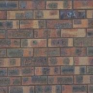
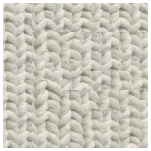
Sample
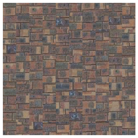
Resultout_size = 300patch_size = 30
The output images did resembled the texture of the source image, but the seams between patches in the grids are clearly visible, and most neighboring patches did not connect at all.
Overlapping Patches
To solve the discontinuities, instead of choosing each patch randomly, each next patch should be similar to the neighboring patches, which the similarity can be solved using the
sum of squared differences (SSD). The new function quilt_simple(sample, out_size, patch_size, overlap, tol) starts by sampling a random patch for the upper-left corner. For all further patches
in the grid, the function will overlap them on top of the existing patches by overlap pixels. To select the next patch,
the function calculates the SSD costs between the overlap-wide overlapping region and all possible patches in the source image, and choose one of the tol patches that
have the smallest SSD costs. The goal of this selection algorithm is to minimize the discontinuities in the output image while preserving enough randomness such that the result feels natural.
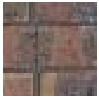
Sample 1
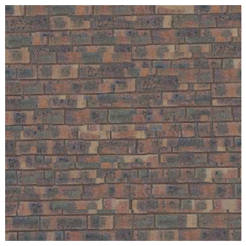
Resultout_size = 300patch_size = 40overlap = 20tol = 20
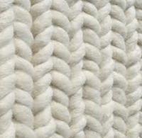
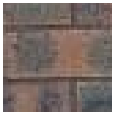
Sample 2
Resultout_size = 300patch_size = 40overlap = 20tol = 10
Since patches are chosen with some guidance, the output images of quilt_simple felt more connected. However, noticible edge artifacts still presented between many patches.
Seam Finding
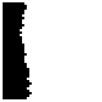
One way to remove edge artifacts from the overlapping patches is the seam finding technique. For each newly sampled patch in the quilt_cut function, this technique finds a contiguous path from the left-to-right and up-to-down
sides of the patch, that minimizes the square differences of the existing output image and the newly sampled patch along the path.
Below is a visulization of the technique on a single patch.
Existing Output Image
Newly Sampled Patch
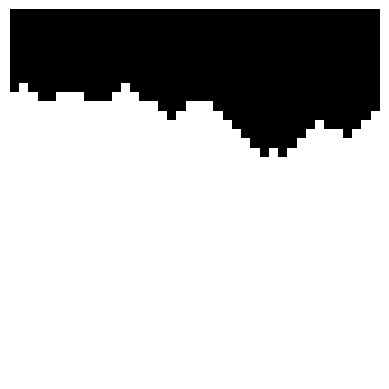
Horizontal Path
Vertical Path
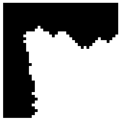
Combined Path
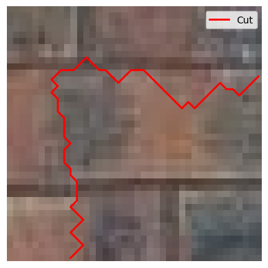
Blended Patch with Cut
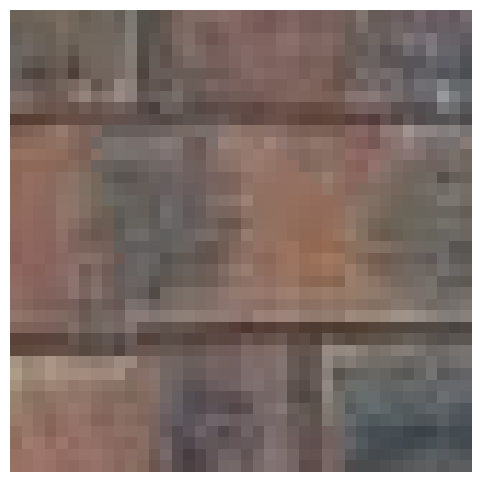
Blended Patch
As shown in the visulization, by making this path a mask and overlap the new patch base on this mask, this technique smooths out the seams between patches, and thus makes the output images seem more connected.
Sample 1
Resultout_size = 300patch_size = 30overlap = 20tol = 20
Sample 2
Resultout_size = 300patch_size = 30overlap = 20tol = 20
Texture Transfer
The quilt_cut function in the last part can also be used to perform texture transfer, which in addition to synthesize texture from a source image, uses an additional guidance image to guide the structure of the output image, thus
"transfering" the texture from the source image to the guidance image.
To implement this texture_transfer function, instead of calculating the SSD costs between the overlapping region and the source image, it also calculates the SSD costs between the overlapping region and the guidance image, and
combine two costs based on the alpha parameter, such that cost = alpha * cost_source + (1 - alpha) * cost_guidance.
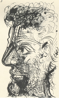
Sketch
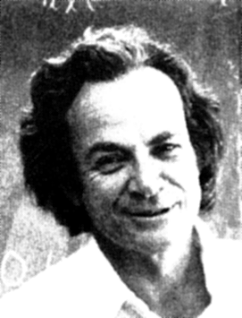
Feynman
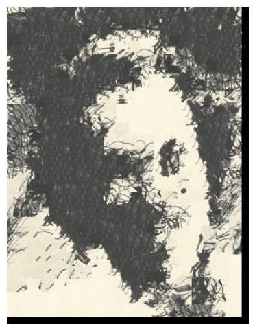
Feynman with Sketch Texturealpha = 0.25patch_size = 25overlap = 11tol = 20
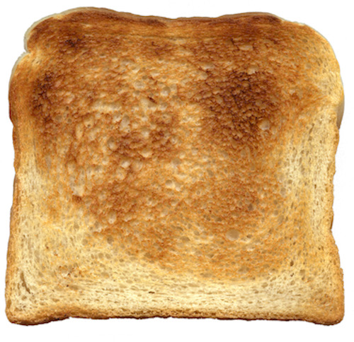
Toast
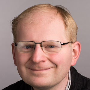
Efros
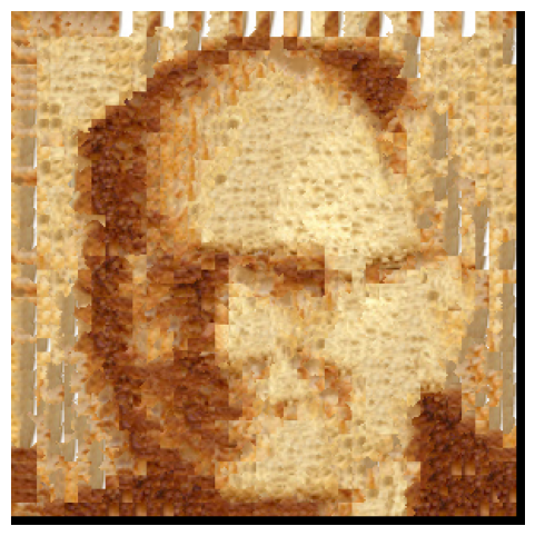
Efros with Toast Texture (Efroast)alpha = 0.2patch_size = 15overlap = 7tol = 20
Gradient Domain Fusion
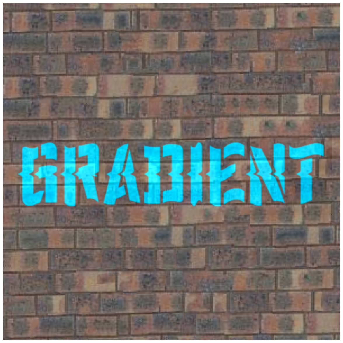
When naively overlap an image onto another, the seams in the overlapping region and the background differences are clearly noticible. This part of the project focused on Poisson blending, a technique that seamlessly blend an object from a source image into the target image.
Toy Problem
Starting with a toy example, an image can be reconstructed from its gradient values and one pixel intensity only.
Let \(s(x, y)\) be the intensity of the source image at \((x, y)\), and the value to solve for as \(v(x, y)\).
For each pixel, there are two objectives:
- Minimize \((v(x+1,y)-v(x,y) - (s(x+1,y)-s(x,y)))^2\) such that the \(x\)-gradients of \(v\) should closely match the \(x\)-gradients of \(s\).
- Minimize \((v(x,y+1)-v(x,y) - (s(x,y+1)-s(x,y)))^2\) such that the \(y\)-gradients of \(v\) should closely match the \(y\)-gradients of \(s\).
To make sure that the reconstructed image resemble the source image, one pixel intensity must be specified as a reference, therefore one more objective is
- Minimize \((v(1,1)-s(1,1))^2\) such that the top left corners of the two images should be the same intensity.
Writing all objective functions as a set of least squares constraints and solve for this optimization, the least squares solution indeed recover the original image.
Source Image
Reconstructed Image
Poisson Blending
Extending on the toy problem, the actual Poisson blending technique blend an object from a source image into the target image seamlessly by calculating intensity values for the target pixels that maximally preserve the gradient of the source object with minimum change, which can be written as the following blending constraints for each pixel. \[ \mathbf{v} = \arg\min_{\mathbf{v}} \left( \sum_{i \in S, j \in \mathcal{N}_i \cap S} \left( (v_i - v_j) - (s_i - s_j) \right)^2 + \sum_{i \in S, j \in \mathcal{N}_i \cap \neg S} \left( (v_i - t_j) - (s_i - s_j) \right)^2 \right) \] Each \(i\) is a pixel in the source region \(S\), and each \(j\) is the 4-neighbor of the corresponding \(i\). The first summation term constraints on the similarity between gradients in \(S\) and the source image, and the second term constraints on the similarity between gradients in the boundary of \(S\) and the target image.
Source Image
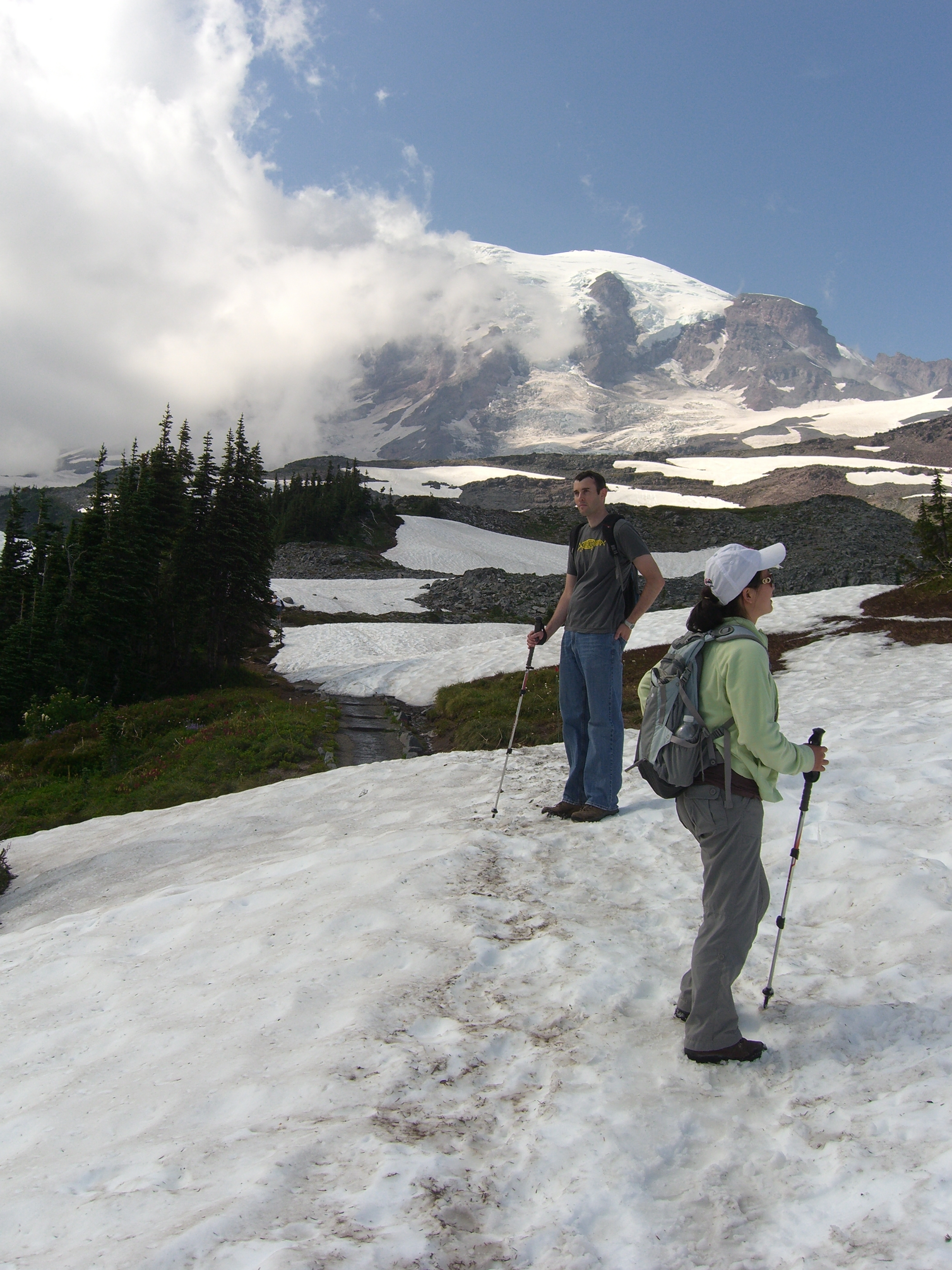
Target Image
Overlap

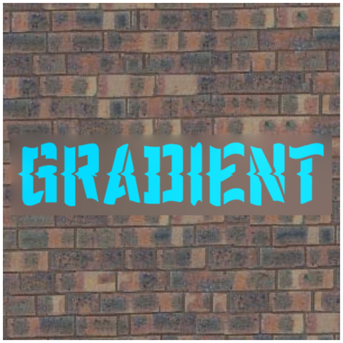
Poisson Blending Result
Source Image
Target Image
Poisson Blending Result
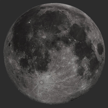
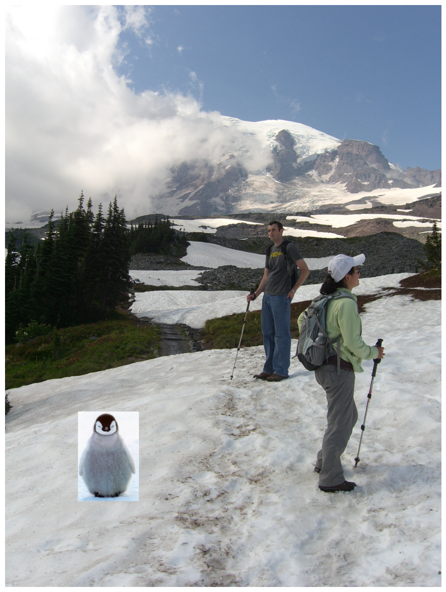
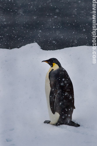
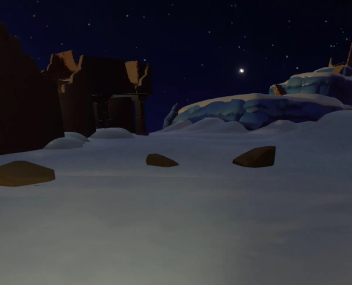
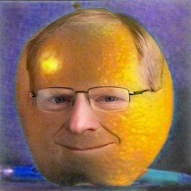
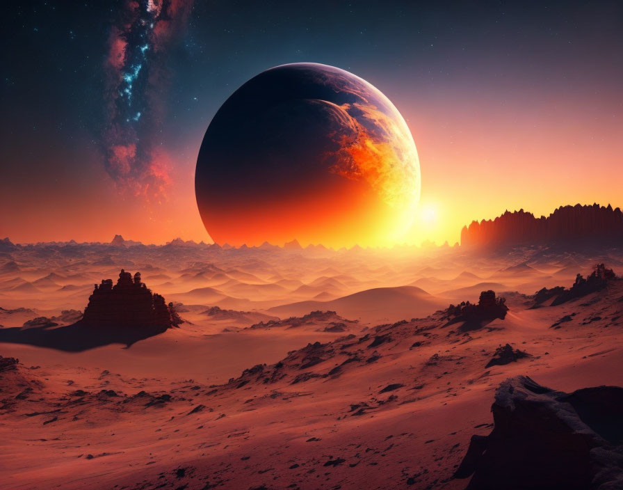
Source Image
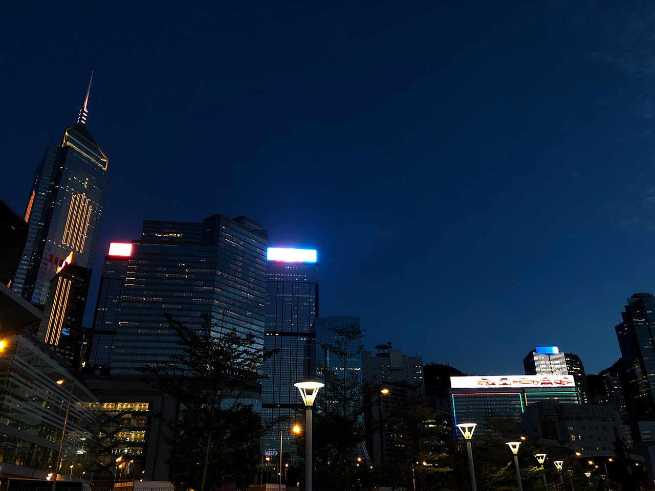
Target Image
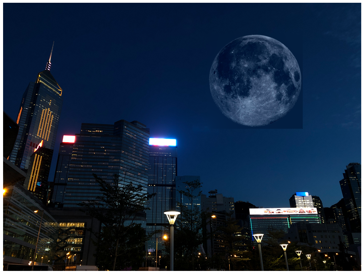
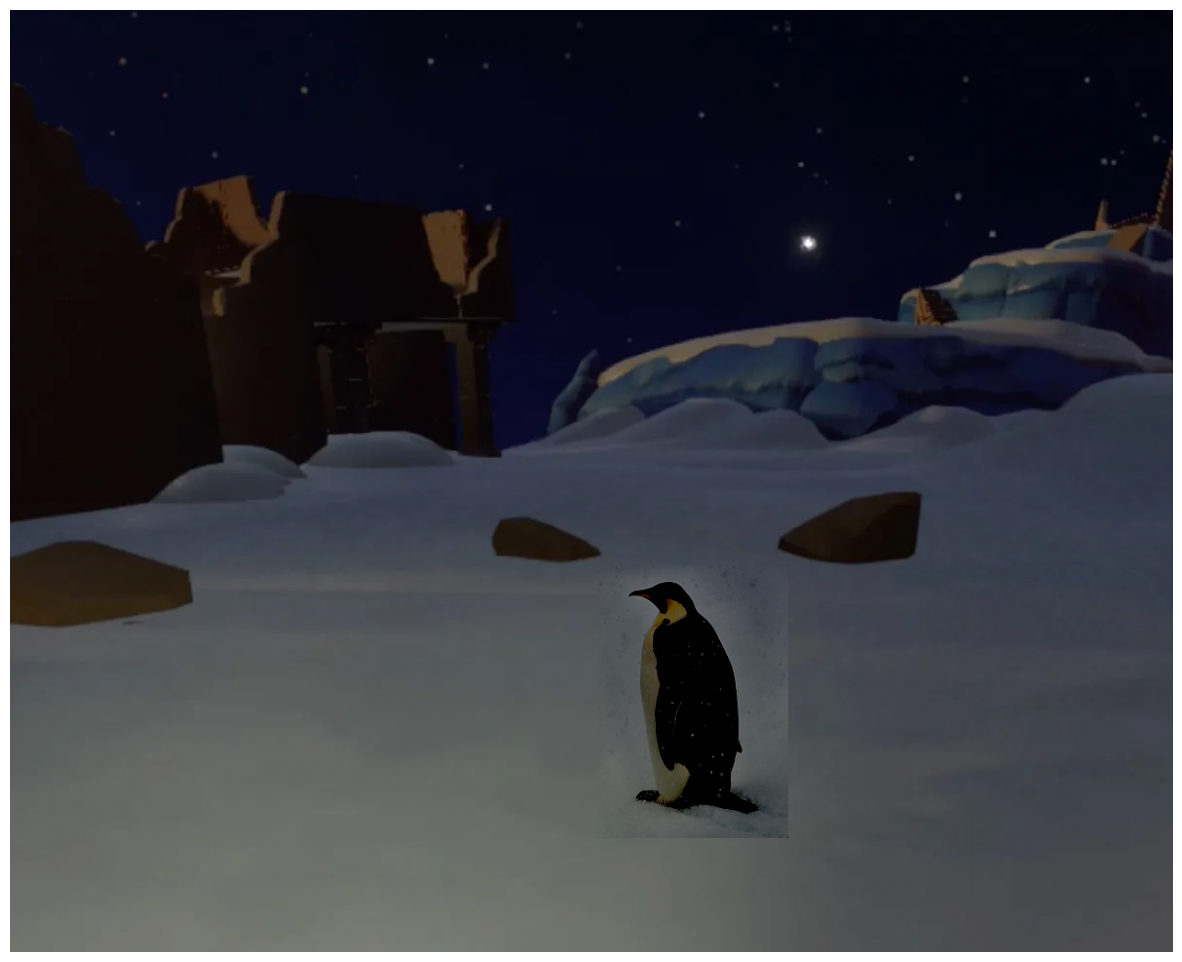
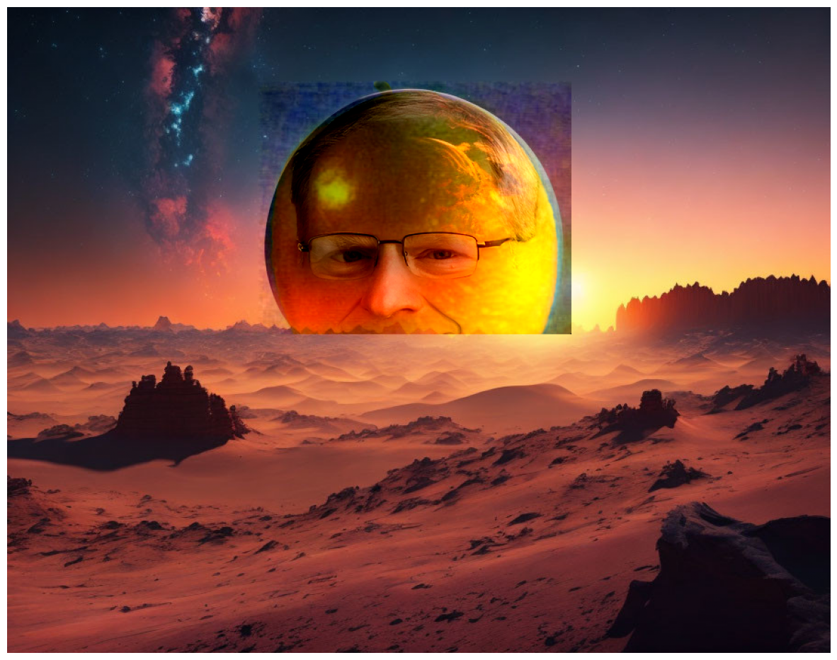
Poisson Blending Result
A side effect of this technique is that the overall intensities are ignored, such that the object might change in color after blending. The technique also performs best only when the background of the object in the source region and the surronding area of the target region have a similar color. As seen in the last result, the color of the moon changed significantly due to the differences between two background colors.
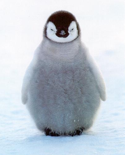
Bells & Whistles: Mixed Gradients
Instead of using the source gradient \((s_i - s_j)\) term in the blending constraints as the only guide, I also tried the following \[ \mathbf{v} = \arg\min_{\mathbf{v}} \left( \sum_{i \in S, j \in \mathcal{N}_i \cap S} \left( (v_i - v_j) - d_{ij} \right)^2 + \sum_{i \in S, j \in \mathcal{N}_i \cap \neg S} \left( (v_i - t_j) - d_{ij} \right)^2 \right) \] where \(d_{ij}\) is the value of the gradient from the source image \((s_i - s_j)\) or the target image \((t_i - t_j)\) with larger magnitude. This will use the gradient in source or target with the larger magnitude as the guide.
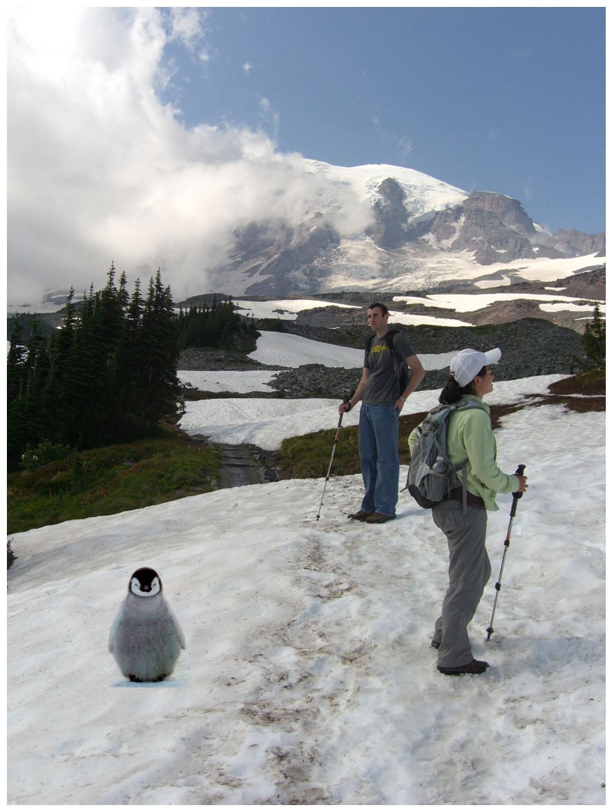
Mixed Gradients Result
Poisson Blending Result from Last Part
Notice that this result with mixed gradients blends the penguin with the background better than the last part. The mixed gradient term in the blending constraints essentially make the source image with a relatively plain background semitransparent. Below are some more blending results that benefits from this feature.
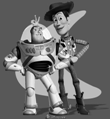
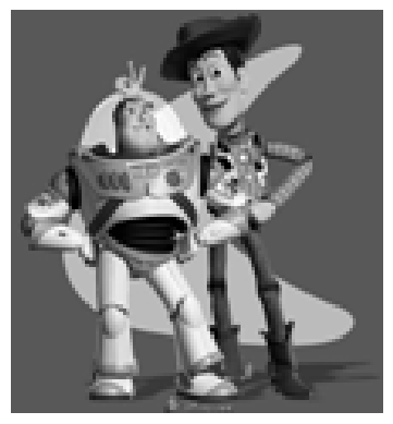
Source Image
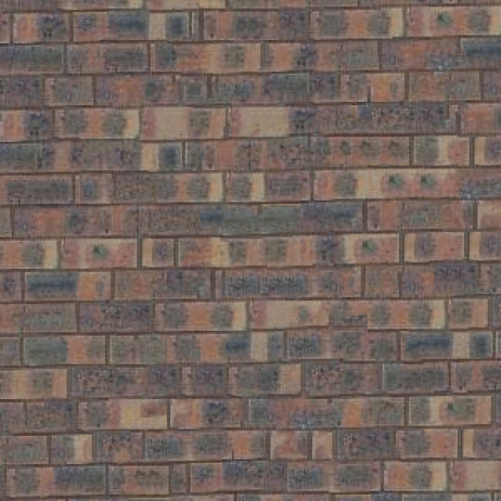
Target Image
Mixed Gradients Result
Poisson Blending Result from Last Part
Source Image
Target Image
Mixed Gradients Result